>Clean and Tidy Data

> When you get new data, you have to clean and organize them. Cleaning new data helps you exploring their content and structure

\ Otho Mantegazza _ Dataviz for Scientists _ Part 1.5

Which Dataset is Tidy?

A common practical way to structure (empirical) data.

Every column is a variable.
Every row is an observation.
Every cell is a single value.
(Every observational unit is in its own table).

Plus: fixed variables should come first, followed by measured variables.

Reference: An Introduction to Tidy Data

Which Dataset is Tidy?

Source: R4DS - Tidy Data

Joey

Monica

Rachel

Phoebe

Ross

Chandler

Tribbiani

Geller

Green

Buffay

Geller

Bing

Semantics of (tidy) Data

Always quoting the Tidy Data article:

A dataset is a collection of values.
Every value belongs to a variable and an observation.
A variable contains all values that measure the same underlying attribute (like height, temperature, duration) across units.
An observation contains all values measured on the same unit (like a person, or a day, or a race) across attributes.

Tools: Tidy data with Tidyr

Tidyr provides functions for:

Pivoting data.
Rectangling data.
Nesting data.
Combining and splitting columns.
Make missing values explicit.

Tidy Pangea Data

Remember the dataset from Pangaea?

pangaea_filename <- 'Dataset_S2_HCl-leaching.tab'

pangaea_path <- 
  here(
    'data/Wu-etal_2022/datasets',
    pangaea_filename
  )

pangaea_data <- 
  pangaea_path %>% 
  read_delim(delim = '\t',
             skip = 49)

Tidy Pangea Data

pangaea_data %>% 
  glimpse()

Rows: 128
Columns: 19
$ Event                      <chr> "SL73BC", "SL73BC", "SL73BC", "SL73BC", "SL…
$ Latitude                   <dbl> 39.6617, 39.6617, 39.6617, 39.6617, 39.6617…
$ Longitude                  <dbl> 24.5117, 24.5117, 24.5117, 24.5117, 24.5117…
$ `Elevation [m]`            <dbl> -339, -339, -339, -339, -339, -339, -339, -…
$ `Sample label (barite-Sr)` <chr> "SL73-1", "SL73-2", "SL73-3", "SL73-4", "SL…
$ `Samp type`                <chr> "non-S1", "non-S1", "non-S1", "S1b", "S1b",…
$ `Depth [m]`                <dbl> 0.0045, 0.0465, 0.0665, 0.1215, 0.1765, 0.1…
$ `Age [ka BP]`              <dbl> 1.66, 3.13, 4.13, 5.75, 7.30, 7.78, 8.65, 9…
$ `CaCO3 [%]`                <dbl> 61.5, 55.1, 53.0, 43.4, 41.8, 42.3, 42.6, 3…
$ `Ba [µg/g] (Leachate)`     <dbl> 72.6, 64.3, 37.4, 63.5, 101.0, 141.0, 75.2,…
$ `Sr [µg/g] (Leachate)`     <dbl> 767, 681, 690, 552, 527, 528, 551, 482, 391…
$ `Ca [µg/g] (Leachate)`     <dbl> 188951.9, 163260.4, 162188.7, 125937.6, 124…
$ `Al [µg/g] (Leachate)`     <dbl> 10612.7, 11428.4, 5463.0, 3261.5, 2121.7, 1…
$ `Fe [µg/g] (Leachate)`     <dbl> 5935.0, 6814.3, 2465.7, 3936.8, 189.6, 7711…
$ `Ba [µg/g] (Residue)`      <dbl> 171.0, 198.0, 251.0, 290.0, 315.0, 259.0, 3…
$ `Sr [µg/g] (Residue)`      <dbl> 66.6, 71.3, 90.3, 99.8, 106.0, 90.7, 108.0,…
$ `Ca [µg/g] (Residue)`      <dbl> 2315.5, 2369.6, 3007.7, 3447.9, 3713.2, 331…
$ `Al [µg/g] (Residue)`      <dbl> 29262.5, 35561.4, 45862.4, 52485.6, 55083.0…
$ `Fe [µg/g] (Residue)`      <dbl> 14834.8, 18301.4, 24534.5, 30745.3, 28532.2…

Better Column Names

we can remove capitalization, spaces, and strange characters from the column names with the function clean_names() from the Janitor Package.

pangaea_data <- 
  pangaea_data %>% 
  janitor::clean_names()

Better Column Names

pangaea_data %>%
  glimpse()

Rows: 128
Columns: 19
$ event                  <chr> "SL73BC", "SL73BC", "SL73BC", "SL73BC", "SL73BC…
$ latitude               <dbl> 39.6617, 39.6617, 39.6617, 39.6617, 39.6617, 39…
$ longitude              <dbl> 24.5117, 24.5117, 24.5117, 24.5117, 24.5117, 24…
$ elevation_m            <dbl> -339, -339, -339, -339, -339, -339, -339, -339,…
$ sample_label_barite_sr <chr> "SL73-1", "SL73-2", "SL73-3", "SL73-4", "SL73-5…
$ samp_type              <chr> "non-S1", "non-S1", "non-S1", "S1b", "S1b", "S1…
$ depth_m                <dbl> 0.0045, 0.0465, 0.0665, 0.1215, 0.1765, 0.1915,…
$ age_ka_bp              <dbl> 1.66, 3.13, 4.13, 5.75, 7.30, 7.78, 8.65, 9.94,…
$ ca_co3_percent         <dbl> 61.5, 55.1, 53.0, 43.4, 41.8, 42.3, 42.6, 39.1,…
$ ba_mg_g_leachate       <dbl> 72.6, 64.3, 37.4, 63.5, 101.0, 141.0, 75.2, 99.…
$ sr_mg_g_leachate       <dbl> 767, 681, 690, 552, 527, 528, 551, 482, 391, 70…
$ ca_mg_g_leachate       <dbl> 188951.9, 163260.4, 162188.7, 125937.6, 124733.…
$ al_mg_g_leachate       <dbl> 10612.7, 11428.4, 5463.0, 3261.5, 2121.7, 12740…
$ fe_mg_g_leachate       <dbl> 5935.0, 6814.3, 2465.7, 3936.8, 189.6, 7711.3, …
$ ba_mg_g_residue        <dbl> 171.0, 198.0, 251.0, 290.0, 315.0, 259.0, 310.0…
$ sr_mg_g_residue        <dbl> 66.6, 71.3, 90.3, 99.8, 106.0, 90.7, 108.0, 96.…
$ ca_mg_g_residue        <dbl> 2315.5, 2369.6, 3007.7, 3447.9, 3713.2, 3316.7,…
$ al_mg_g_residue        <dbl> 29262.5, 35561.4, 45862.4, 52485.6, 55083.0, 44…
$ fe_mg_g_residue        <dbl> 14834.8, 18301.4, 24534.5, 30745.3, 28532.2, 22…

Better Column Names

Watch out: Janitor transforms µ into m (so micrograms become milligrams).

Micrograms on grams is also known as part per million, ppm.

pangaea_data <- 
  pangaea_data %>% 
  rename_all(
    ~str_replace(., 'mg_g', 'ppm')
  )

Fixed Variables in Front

Which column is a fixed variable?

I’m not sure if ca_co3_percent is a measured variable, and if it belongs to another informational unit.

Besides that, the fixed variables are already in front.

Pivot Longer

Source : R4DS - Tidy Data

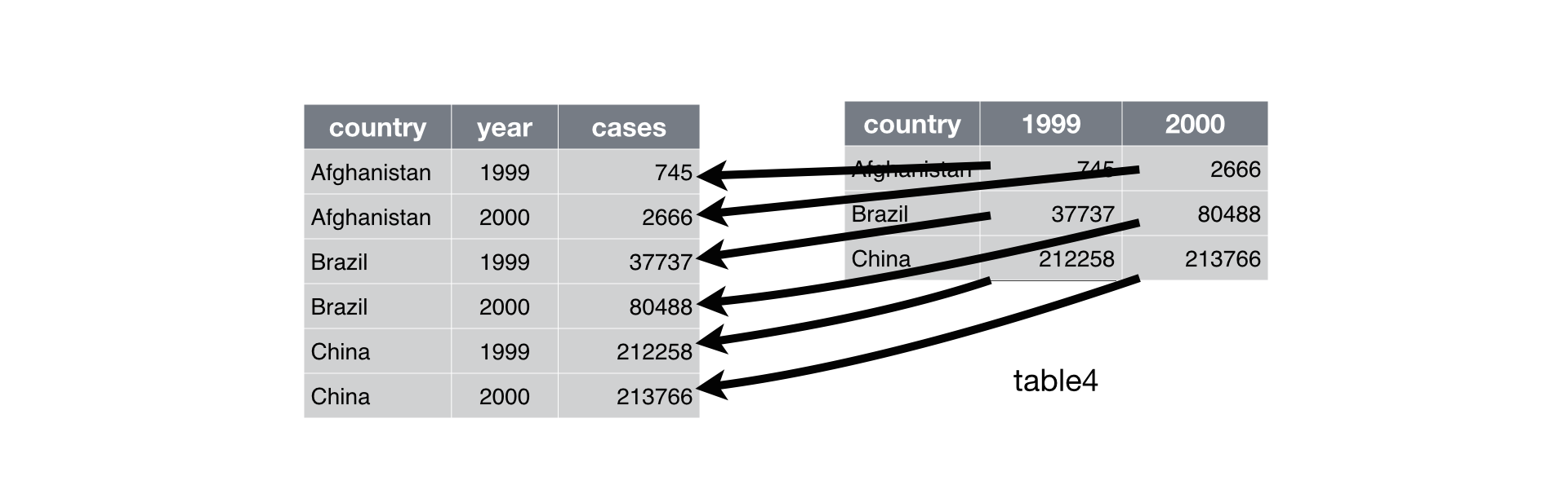
No Values in Column Names

Let’s pivot the measured variables.

pangaea_long <- 
  pangaea_data %>% 
  pivot_longer(
    cols = contains(match = c('leachate', 'residue')),
    values_to = 'concentration',
    names_to = 'element'
  )

No Values in Column Names

When we pivot data we move them from a wide to a long format and vice-versa.

pangaea_long %>% 
  glimpse()

Rows: 1,280
Columns: 11
$ event                  <chr> "SL73BC", "SL73BC", "SL73BC", "SL73BC", "SL73BC…
$ latitude               <dbl> 39.6617, 39.6617, 39.6617, 39.6617, 39.6617, 39…
$ longitude              <dbl> 24.5117, 24.5117, 24.5117, 24.5117, 24.5117, 24…
$ elevation_m            <dbl> -339, -339, -339, -339, -339, -339, -339, -339,…
$ sample_label_barite_sr <chr> "SL73-1", "SL73-1", "SL73-1", "SL73-1", "SL73-1…
$ samp_type              <chr> "non-S1", "non-S1", "non-S1", "non-S1", "non-S1…
$ depth_m                <dbl> 0.0045, 0.0045, 0.0045, 0.0045, 0.0045, 0.0045,…
$ age_ka_bp              <dbl> 1.66, 1.66, 1.66, 1.66, 1.66, 1.66, 1.66, 1.66,…
$ ca_co3_percent         <dbl> 61.5, 61.5, 61.5, 61.5, 61.5, 61.5, 61.5, 61.5,…
$ element                <chr> "ba_ppm_leachate", "sr_ppm_leachate", "ca_ppm_l…
$ concentration          <dbl> 72.6, 767.0, 188951.9, 10612.7, 5935.0, 171.0, …

One Value Per Cell

Now it’s clear that element contains more than one value.

For example: ba_ppm_leachate is not a single values and could be split into:

element: ba.
unit: **ppm*.
fraction: leachate.

Let’s split this column at the **_** and reconstitute it in a tidy way

One Value Per Cell

pangaea_tidy <- 
  pangaea_long %>% 
  separate(element, 
           into = c(
             'element', 
             'unit', 
             'fraction'
           ),
           sep = '_')

One Value Per Cell

pangaea_tidy %>% glimpse()

Rows: 1,280
Columns: 13
$ event                  <chr> "SL73BC", "SL73BC", "SL73BC", "SL73BC", "SL73BC…
$ latitude               <dbl> 39.6617, 39.6617, 39.6617, 39.6617, 39.6617, 39…
$ longitude              <dbl> 24.5117, 24.5117, 24.5117, 24.5117, 24.5117, 24…
$ elevation_m            <dbl> -339, -339, -339, -339, -339, -339, -339, -339,…
$ sample_label_barite_sr <chr> "SL73-1", "SL73-1", "SL73-1", "SL73-1", "SL73-1…
$ samp_type              <chr> "non-S1", "non-S1", "non-S1", "non-S1", "non-S1…
$ depth_m                <dbl> 0.0045, 0.0045, 0.0045, 0.0045, 0.0045, 0.0045,…
$ age_ka_bp              <dbl> 1.66, 1.66, 1.66, 1.66, 1.66, 1.66, 1.66, 1.66,…
$ ca_co3_percent         <dbl> 61.5, 61.5, 61.5, 61.5, 61.5, 61.5, 61.5, 61.5,…
$ element                <chr> "ba", "sr", "ca", "al", "fe", "ba", "sr", "ca",…
$ unit                   <chr> "ppm", "ppm", "ppm", "ppm", "ppm", "ppm", "ppm"…
$ fraction               <chr> "leachate", "leachate", "leachate", "leachate",…
$ concentration          <dbl> 72.6, 767.0, 188951.9, 10612.7, 5935.0, 171.0, …

Data can take many shapes

pangaea_also_tidy <- 
  pangaea_tidy %>% 
  pivot_wider(names_from = 'element', values_from = 'concentration')

Data can take many shapes

pangaea_also_tidy %>% glimpse()

Rows: 256
Columns: 16
$ event                  <chr> "SL73BC", "SL73BC", "SL73BC", "SL73BC", "SL73BC…
$ latitude               <dbl> 39.6617, 39.6617, 39.6617, 39.6617, 39.6617, 39…
$ longitude              <dbl> 24.5117, 24.5117, 24.5117, 24.5117, 24.5117, 24…
$ elevation_m            <dbl> -339, -339, -339, -339, -339, -339, -339, -339,…
$ sample_label_barite_sr <chr> "SL73-1", "SL73-1", "SL73-2", "SL73-2", "SL73-3…
$ samp_type              <chr> "non-S1", "non-S1", "non-S1", "non-S1", "non-S1…
$ depth_m                <dbl> 0.0045, 0.0045, 0.0465, 0.0465, 0.0665, 0.0665,…
$ age_ka_bp              <dbl> 1.66, 1.66, 3.13, 3.13, 4.13, 4.13, 5.75, 5.75,…
$ ca_co3_percent         <dbl> 61.5, 61.5, 55.1, 55.1, 53.0, 53.0, 43.4, 43.4,…
$ unit                   <chr> "ppm", "ppm", "ppm", "ppm", "ppm", "ppm", "ppm"…
$ fraction               <chr> "leachate", "residue", "leachate", "residue", "…
$ ba                     <dbl> 72.6, 171.0, 64.3, 198.0, 37.4, 251.0, 63.5, 29…
$ sr                     <dbl> 767.0, 66.6, 681.0, 71.3, 690.0, 90.3, 552.0, 9…
$ ca                     <dbl> 188951.9, 2315.5, 163260.4, 2369.6, 162188.7, 3…
$ al                     <dbl> 10612.7, 29262.5, 11428.4, 35561.4, 5463.0, 458…
$ fe                     <dbl> 5935.0, 14834.8, 6814.3, 18301.4, 2465.7, 24534…

Pivot Wider

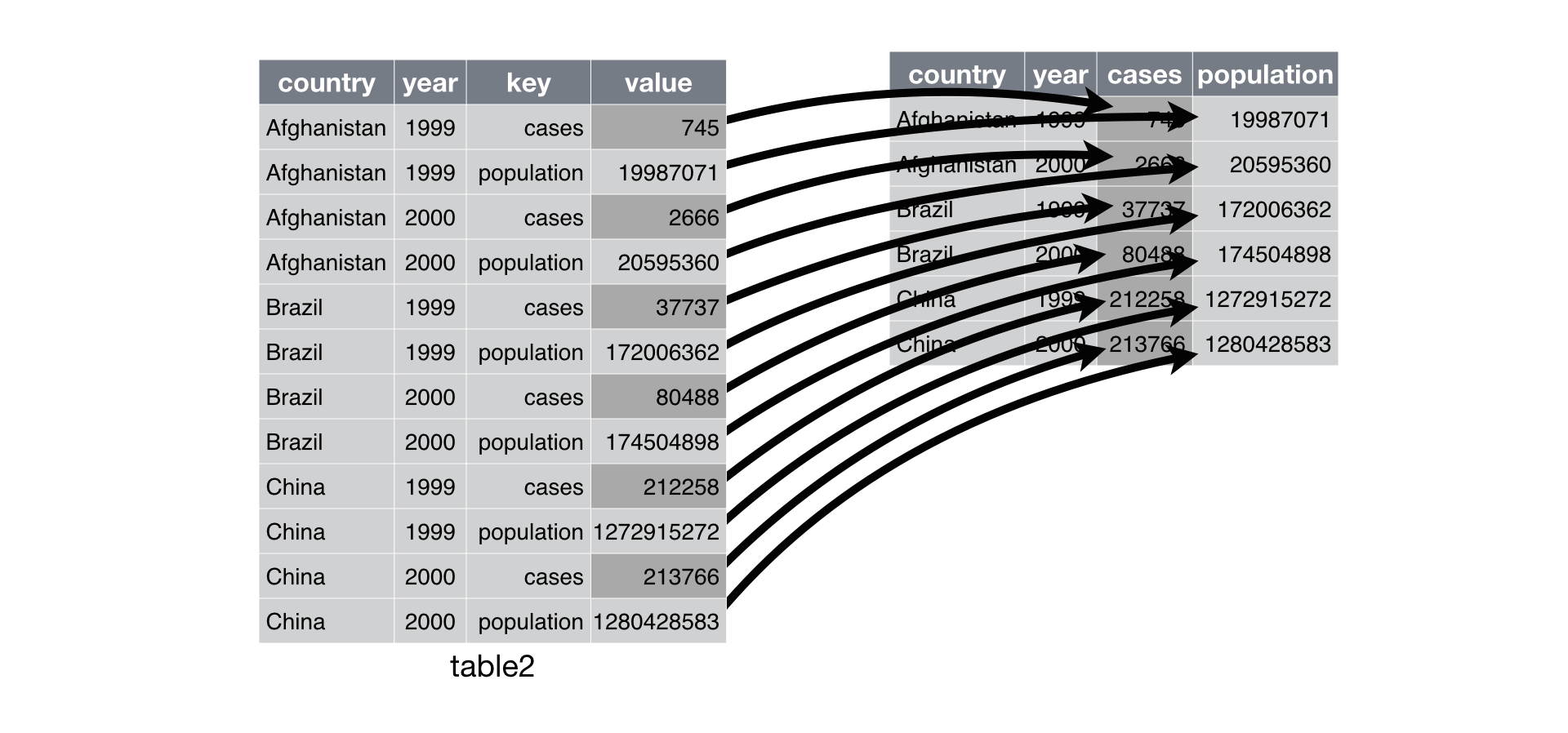
Source : R4DS - Tidy Data

Exercise

Tidy the iris dataset:

iris %>% 
  as_tibble()

# A tibble: 150 × 5
   Sepal.Length Sepal.Width Petal.Length Petal.Width Species
          <dbl>       <dbl>        <dbl>       <dbl> <fct>  
 1          5.1         3.5          1.4         0.2 setosa 
 2          4.9         3            1.4         0.2 setosa 
 3          4.7         3.2          1.3         0.2 setosa 
 4          4.6         3.1          1.5         0.2 setosa 
 5          5           3.6          1.4         0.2 setosa 
 6          5.4         3.9          1.7         0.4 setosa 
 7          4.6         3.4          1.4         0.3 setosa 
 8          5           3.4          1.5         0.2 setosa 
 9          4.4         2.9          1.4         0.2 setosa 
10          4.9         3.1          1.5         0.1 setosa 
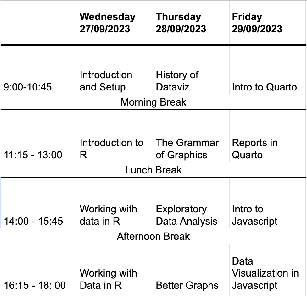
# ℹ 140 more rows

Exercise

Tidy last week’s schedule: